Machine Learning in Practice: My Journey Building the Tanzania Tourism Expenditure Classifier
In machine learning, we love to talk about accuracy. But accuracy only tells you whether a model was right, not how sure it was. Over four days in September 2026, I took part in a hackathon that scored us on something far less forgiving.
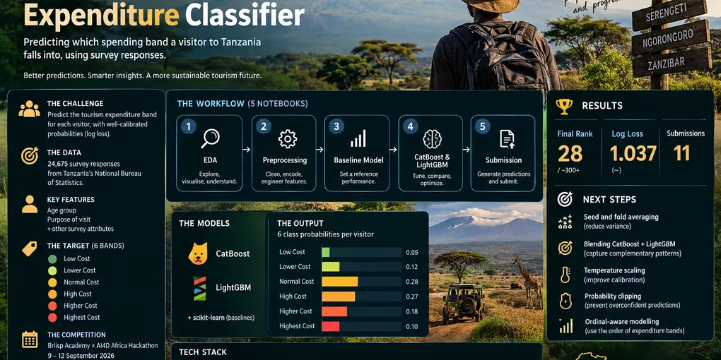
Hosted by Briisp Academy and the AI4D Africa Anglophone Multidisciplinary Research Lab, the challenge was open to university students across English-speaking African countries. It asked one question: given a tourist’s survey answers, how much will they spend in Tanzania? Tourism makes up roughly 17% of the country’s GDP, so a good answer is useful to tour operators and the Tanzania Tourism Board alike. Here is how I built my solution and what I learned along the way.

Wildebeest migration in Serengeti National Park, Tanzania. Photo via Wikimedia Commons, licensed under CC BY 4.0. [Add the photographer’s name from the file page.]

The Challenge: Six Bands, One Metric
The dataset contains 24,675 survey responses collected by Tanzania’s National Bureau of Statistics. Each row describes a visitor: their age group, their purpose of visit (business, leisure, volunteering, visiting friends and family) and other travel characteristics. The job was to place each visitor into one of six expenditure bands:
- Low Cost
- Lower Cost
- Normal Cost
- High Cost
- Higher Cost
- Highest Cost
Notice that these bands have a natural order. A “High Cost” visitor is closer to “Higher Cost” than to “Low Cost”. That detail matters, and I come back to it at the end.
Why Log Loss Is a Different Game
Submissions were not scored on how many visitors I placed in the right band. They were scored on log loss, which means I had to submit six probabilities for every visitor, and the score punished me according to how much probability I gave to the true band.
A quick way to feel the difference: if the correct band gets a probability of 0.9, the penalty is about 0.11. If it gets 0.1, the penalty jumps to about 2.3. And if I had been 99% sure of the wrong answer and left just 1% on the truth, the penalty would be about 4.6. A handful of overconfident mistakes can undo the work of thousands of good predictions.
For scale, a model that spreads probability evenly across all six bands scores about 1.79. Every serious entry on the leaderboard sat well below that, so the fight was about squeezing out small, honest improvements in calibration.
The Vision: More Than Just a Prediction
Most beginners fit a model, check the accuracy and submit. My goal was to treat this like a real ML product. I wanted a workflow that:
- Started simple: A baseline model first, so every later idea had something to beat.
- Reproduced itself: A pinned environment so the project runs the same on any machine.
- Spoke in probabilities: Six probability columns per visitor, in a fixed and documented order, not just a single guess.
- Stayed honest: Local validation that used the same metric as the leaderboard.
The Architecture: How I Built It
1. The Notebook Pipeline
I split the work into five numbered notebooks, run in order, so anyone (including future me) can follow the story from raw data to final submission:
01_eda.ipynb– Exploratory analysis. This is where I looked at how the six bands were distributed, checked missing values, and studied how features like age group and purpose of visit relate to spending.02_preprocessing.ipynb– Cleaning and feature preparation. Anything that would be applied to the training data had to be reproducible on the test data, so this notebook kept those steps in one place.03_baseline_model.ipynb– The benchmark. A deliberately simple model that gave me a first log loss score and a working submission file early on.04_modelling.ipynb– Training and comparing candidate models. [Describe your final model and any features you engineered.]05_submission.ipynb– Generating predictions and writing the six probability columns in the exact class order the competition required.
2. The Technical Stack
I chose tools that suit tabular survey data and that I could trust to be reproducible:
- Python (Pandas & NumPy): My workhorse for cleaning and transforming the survey responses.
- CatBoost: A gradient boosting library with strong native support for categorical features, which is exactly what survey data is full of.
- LightGBM: A fast, memory-efficient gradient boosting library that made it cheap to try many ideas in a short time.
- Scikit-learn: Preprocessing, cross-validation utilities and the log loss metric itself.
- Matplotlib & Plotly: For exploring the data visually before I trusted any model built on it.
- uv & requirements.txt: A locked, pinned environment so the project rebuilds the same way every time.
Key Milestones & “Aha!” Moments
Log Loss Changes Everything
Once I truly understood the metric, my questions changed. I stopped asking “which band is most likely?” and started asking “how confident should I be, and is that confidence earned?” Choosing a model, tuning it and formatting the output all became calibration problems.
The Baseline Pays Off
Building a baseline before anything fancy gave me a reference point and a valid submission on the board early. From then on, every experiment answered a simple question: did the score go down or not? That removed a lot of guesswork.
Eleven Submissions, One Tight Leaderboard
Across the four days I made 11 submissions and finished at rank 28 with a private score (log loss) of about 1.037. The leaderboard shows two scores: a public score, visible while the competition ran, and a private score computed on the held-out remainder of the test data. The final ranking follows the private score. My public score was about 1.058.
The winner finished with a private log loss of about 1.030, so I was roughly 0.007 behind first place. What stood out was how compressed the whole board was. The top three were separated by less than 0.0005, and the top ten all fell within 0.003.
| Reference point | Private log loss |
|---|---|
| Rank 1 | about 1.030 |
| Rank 17 | about 1.035 |
| My score (rank 28) | about 1.037 |
| Rank 40 | about 1.043 |
| Guessing all six bands equally | about 1.79 |
Two details from the board taught me as much as the scores did:
- Public scores did not predict the final order. The winner’s public score (about 1.051) was worse than several entries that finished below them. The board you see during the competition is only a partial picture.
- More submissions did not mean a better rank. The top spot took 66 submissions, but a couple of top-ten finishers made just one.
In a field this tight, improvements live in the third and fourth decimal places, and it becomes hard to tell real progress from noise.
Lessons Learned (The Hard Way)
1. The Metric Is the Brief
Log loss shaped every decision, from model choice to how I formatted the submission. It rewards being appropriately unsure, so a model that is slightly less “accurate” but better calibrated can win. Reading the evaluation rules carefully on day one was the best investment I made.
2. Baseline First, Always
Progress means nothing without something to compare it to. A simple baseline told me how much of the signal was easy to capture, and it made every later gain feel earned rather than imagined.
3. Trust Validation Over the Leaderboard
With 11 submissions and scores that differed in the fourth decimal place, it was tempting to chase the leaderboard. But a leaderboard is one slice of data, and small gaps can be noise. Cross-validation on the training data is a far more honest guide, and I learned to treat a leaderboard jump as a hint rather than a verdict. The public and private boards made this concrete for me: my public score was about 1.058, my private score about 1.037, and the order on the public board did not match the final order.
4. Understand the Data Before Modelling
Survey data is human data: answers are categorical, some may be missing, and some categories are rare. Time spent in the EDA notebook made every later step easier, because I knew what the columns meant and where the model could go wrong. Better models can’t rescue data you don’t understand.
5. Respect Your Categorical Features
Most of what a tourist survey captures is categories, not numbers. That is why gradient boosting libraries with good categorical handling, like CatBoost, are such a natural fit. Encoding choices are modelling choices, and they deserve as much thought as the algorithm.
6. Probabilities Are the Product
The output was six numbers per visitor, and each row had to sum to one, in a fixed column order. A mismatch between the class mapping used in training and the order used in the submission would silently wreck the score. I learned to define the mapping once and reuse it everywhere.
7. Structure Saves Time
Numbered notebooks and a pinned environment meant I never wondered what I had already run or which version of a library I used. When the clock is short, not losing time to confusion is a real advantage.
8. Four Days Is Short, So Prioritise
A hackathon rewards focus. Getting a valid baseline submission in early, then spending remaining time on the changes most likely to move log loss, worked better than trying every idea. Knowing what not to try is a skill.
9. A Leaderboard Is a Classroom
The board had participants from across Africa, and seeing how close everyone’s scores were was humbling and motivating at the same time. Competing alongside so many capable students showed me how much I still have to learn, and how much faster you learn when you can measure yourself against others.
What I’d Do Differently Next Time
Looking at where I finished, these are the steps I plan to try in my next challenge. Each is a small change that tends to pay off specifically on log loss.
Average Several Seeds and Folds
A single model trained once can be sensitive to randomness. Averaging predictions from several random seeds, or from models trained on different cross-validation folds, smooths the probabilities and usually lowers log loss.
Blend CatBoost and LightGBM
Two different boosting libraries make different mistakes. A simple weighted average often beats either model on its own:
# Blend two sets of class probabilities (each: n_samples x 6)
blend = 0.5 * cat_probs + 0.5 * lgbm_probs
Calibrate the Outputs
If a model is systematically overconfident, a single “temperature” parameter fitted on out-of-fold predictions can fix it:
import numpy as np
from scipy.optimize import minimize_scalar
from sklearn.metrics import log_loss

def apply_temperature(probs, T):
    logits = np.log(np.clip(probs, 1e-15, 1.0)) / T
    logits -= logits.max(axis=1, keepdims=True)
    exp = np.exp(logits)
    return exp / exp.sum(axis=1, keepdims=True)

def fit_temperature(oof_probs, y_true):
    result = minimize_scalar(
        lambda T: log_loss(y_true, apply_temperature(oof_probs, T), labels=list(range(6))),
        bounds=(0.5, 3.0),
        method="bounded",
    )
    return result.x
Clip Extreme Probabilities
As the log loss example showed, near-zero probabilities on the true class are dangerous. A light clip, followed by renormalising each row, protects against a few overconfident mistakes:
probs = np.clip(probs, 1e-3, 1 - 1e-3)
probs = probs / probs.sum(axis=1, keepdims=True)
Use the Order of the Bands
Because the six bands run from Low Cost to Highest Cost, they are ordinal rather than unrelated labels. Ordinal-aware approaches, or features that reflect that ordering, might extract signal that a plain multiclass model treats as independent categories. I did not get to explore this properly, so it is high on my list.
What’s Next?
This project is the natural follow-up to my Superstore analytics work. That one taught me how to build the pipes; this one taught me how to make predictions I can trust. Next, I want to keep pairing solid engineering habits with models that are honest about their uncertainty. That means better validation, better calibration and a workflow I can reuse on the next challenge.
To everyone at Briisp Academy and AI4D Africa who organised the hackathon, thank you. And to my fellow participants, thank you for a competitive board that pushed me to learn.
Explore the Project
Check out the full codebase and notebooks on my GitHub: Tanzania Tourism Expenditure Classifier Repository